Comparison of A2C and PPO Reinforcement Learning Algorithms
Introduction
Reinforcement learning is a subset of artificial intelligence where agents, the decision makers, interact with an environment to receive a reward and learn optimal behaviors over time to achieve a specific goal. After understanding the foundations of reinforcement learning algorithms throughout this past semester, this post explores two specific reinforcement learning algorithms: Actor Advantage Critic (A2C) and Proximal Policy Optimization (PPO).
These two algorithms are recent breakthroughs in reinforcement learning and aim to solve challenges regarding sample inefficiency and instability of policy updates. To compare these algorithms against one another, I’ll be using the OpenAI Gym CartPole-v1 environment as a basis for performance evaluation.
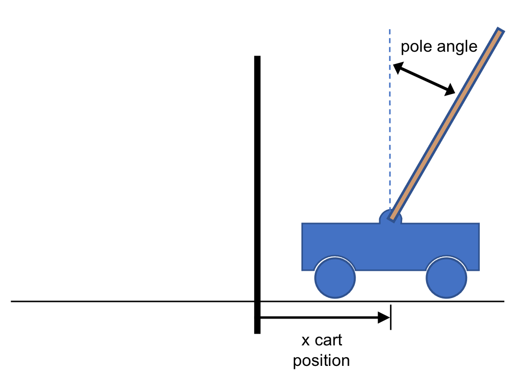
The CartPole-v1 problem is a benchmark that evaluates the agent’s ability to balance a pole against a moving cart by either moving left or right. Let’s explore the theoretical foundations of these algorithms and their practical implementation in the CartPole environment, while comparing their strengths and weaknesses.
Advantage Actor Critic (A2C)
The Advantage Actor Critic algorithm combines an actor-critic system, where the actor selects the action the agent should take based on the current state of the environment, and the critic evaluates the impact of the action by estimating the value of the current state of the environment.
By combining the critic’s feedback with the actor’s decision-making, the critic guides and helps the actor improve its decision making over time. The actor uses an advantage function to determine how much better it is to take a particular action in a state compared to the average value of actions in that state. Moreover, the advantage function serves as a tool to reduce the variance in policy gradients resulting in more stable and efficient updates to the policy.
The advantage function uses both action-value and state-value, emphasizing the quality of the action rather than the quantity of the reward:
\[A(s, a) = Q(s, a) - V(s)\]The A2C algorithm maintains an actor network with parameters $\theta$ and a critic network with parameters $\theta_v$ that share common features.
For each state visited, the actor selects the action according to policy $\pi(a_t | s_t; \theta’)$ and the environment returns a reward and state at timestep $t$. The algorithm then computes a bootstrapped estimate $R$ which is used to accumulate gradients for both actor and critic networks. While the actor’s gradients are scaled by $R - V(s_i; \theta_v’)$ to encourage exploitation, the critic’s gradients are scaled by $(R - V(s_i; \theta_v’))^2$ to minimize errors for predicted state values.
Proximal Policy Optimization (PPO)
The Proximal Policy Optimization is the most recent breakthrough in the field of reinforcement learning and is built upon the previous A2C algorithm discussed above. A2C previously would struggle with stability of large policy changes since there was no method to control the magnitude of policy updates, causing performance decline and slower convergence.
However, PPO approaches this problem by introducing policy update constraints to ensure that the updated policy does not deviate too far from the current policy. PPO solves this problem by utilizing a surrogate objective function with a clipping mechanism which effectively limits the size of the policy updates.
The probability ratio between current and old policies is defined as:
\[r_t(\theta) = \frac{\pi_\theta(a_t | s_t)}{\pi_{old}(a_t | s_t)}\]And the surrogate objective function is:
\[L_t(\theta) = \min(r_t(\theta) \hat{A}_t, \text{clip}(r_t(\theta), 1 - \epsilon, 1 + \epsilon) \hat{A}_t)\]The above surrogate objective function essentially minimizes large or unstable policy changes by penalizing updates if the probability ratio deviates significantly from 1 by clipping the ratio between 1 - ε and 1 + ε, where ε is a set hyperparameter that controls the update range.
Here’s a pseudocode for the PPO algorithm:
1
2
3
4
5
6
7
8
9
Algorithm 1: PPO, Actor-Critic Style
for iteration=1,2,... do
    for actor=1,2,...,N do
        Run policy π_old in environment for T timesteps
        Compute advantage estimates Â_1,...,Â_T
    end for
    Optimize surrogate L wrt θ, with K epochs and minibatch size M ≤ NT
    θ_old ← θ
end for
The PPO algorithm first collects experience using the old policy for a set T timesteps across multiple parallel actors. For each experience, it then computes the advantage function measuring the quality or impact of an action compared to the expected value. The key aspect of PPO is the optimization step using the surrogate function L that is optimized for K epochs with mini batches of size M, effectively constraining policy changes and improving stability.
A2C and PPO CartPole Experiment Setup
To evaluate the performance of both the A2C and PPO algorithms, I utilized OpenAI’s Gymnasium CartPole-v1 environment, which is a classic reinforcement learning control problem where the agent must balance a pole on a moving cart.
The state space for the Cartpole problem consists of four continuous variables:
- Cart position
- Cart velocity
- Pole angle
- Pole angular velocity
The action space consists of two discrete actions: moving the cart left or right. Based on OpenAI’s Gymnasium documentation, the CartPole problem is solved when an average reward of 475 over 100 consecutive episodes is achieved.
Advantage Actor Critic (A2C) Implementation
For the A2C implementation, I developed an Environment class that normalizes the state using a running mean and running standard deviation to improve training stability. The neural network architecture utilizes shared feature layers between the actor and critic with two hidden layers of 64 units each. The actor outputs log-scaled action probabilities using softmax and the critic outputs the state value estimation.
Both actor and critic were optimized using the Adam optimizer with a learning rate of 1e-3. The following hyperparameters were utilized:
- Learning Rate: 1e-3
- Discount Factor γ: 0.99
- Maximum Episode Length: 500 steps
- Maximum Number of Episodes: 1500
- Actions were selected using a categorical probability distribution
Proximal Policy Optimization (PPO) Implementation
The PPO implementation utilized the same Environment wrapper used in the A2C implementation and a similar Actor-Critic setup. PPO’s neural network architecture, however, utilizes two separate network architectures.
The actor network has an input layer of 4 units, representing the state dimension and passes through two fully connected hidden layers, each with a hidden dimension of 64 units and Tanh activations. The output layer produces 2 units, representing the action dimension.
Similarly, the critic network takes the state dimension as input, passes through two hidden layers with Tanh activations, and outputs a single value, representing the estimated state value. The following hyperparameters were utilized:
- Learning rate: 3e-4 (actor) 1e-3 (critic)
- Discount Factor γ: 0.99
- Maximum Episode Length: 500 steps
- Maximum Number of Episodes: 1500
- General Advantage Estimation (GAE): 0.98
- Clip ε: 0.2
- Buffer Size: 4096
- Batch Size: 64
- Number of Epochs: 10
CartPole Results and Comparisons
Both A2C and PPO were able to successfully solve the CartPole-v1 control problem and meet OpenAI’s solving criteria of an average reward of 475 over 100 consecutive episodes, though with differences in their speed of learning.
Whereas A2C solved the CartPole-v1 problem in 930 episodes, the PPO implementation was able to solve the CartPole-v1 problem more efficiently in 560 episodes.
As shown by the figures below, A2C displays a steady improvement with an initial slow learning curve from episodes 0 to 200 with average rewards under 100, followed by a rapid improvement section from episodes 200 to 260 increasing to approximately an average reward of 400, and a final fine-tuning phase from episodes 600 to 930 stabilizing the average reward achieved.
Though PPO solves the CartPole-v1 problem quicker, it has an exploration phase twice as long, from episodes 0 to 400 with consistent low rewards, followed by a steep increase in reward from episodes 200 to 600 with an average reward of approximately 500, and a final fine-tuning phase from episodes 600 to 930.
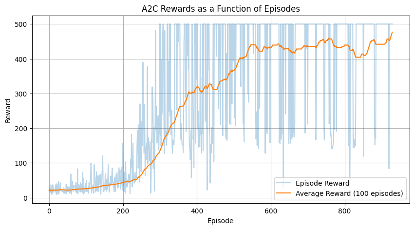 Figure 1: A2C Rewards as a Function of Time
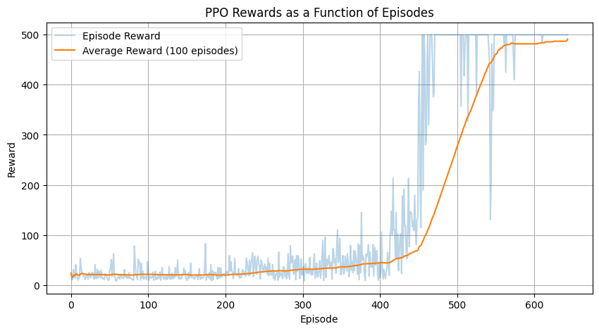 Figure 2: PPO Rewards as a Function of Time
Conclusion
In this post, we compared two modern reinforcement learning algorithms, A2C and PPO, on the CartPole-v1 environment. Both algorithms successfully solved the task, but PPO demonstrated superior sample efficiency by solving the problem in 560 episodes compared to A2C’s 930 episodes.
This efficiency gain can be attributed to PPO’s clipping mechanism that limits policy updates, preventing the large, destabilizing changes that can occur in A2C. This stability allows PPO to make more consistent progress during training.
However, it’s worth noting that A2C showed more gradual and steady improvement, which might be preferable in certain applications where stable, predictable learning progress is more important than raw speed.
In future work, it would be interesting to test these algorithms on more complex environments to better understand their scaling properties and performance characteristics across different types of tasks.
References & Links
Github Source
Here is the source code for the A2C and PPO implementations used in this post: anshul-rao/gym-cartpole.